Numerically exact distortion estimation
and numerically exact undistortion
validated against known ground-truth distortion fields —
available in MATLAB and Python.
The accompanying paper is a draft preprint, in preparation — not yet
peer-reviewed.
Numerically Exact Distortion Estimation NEW
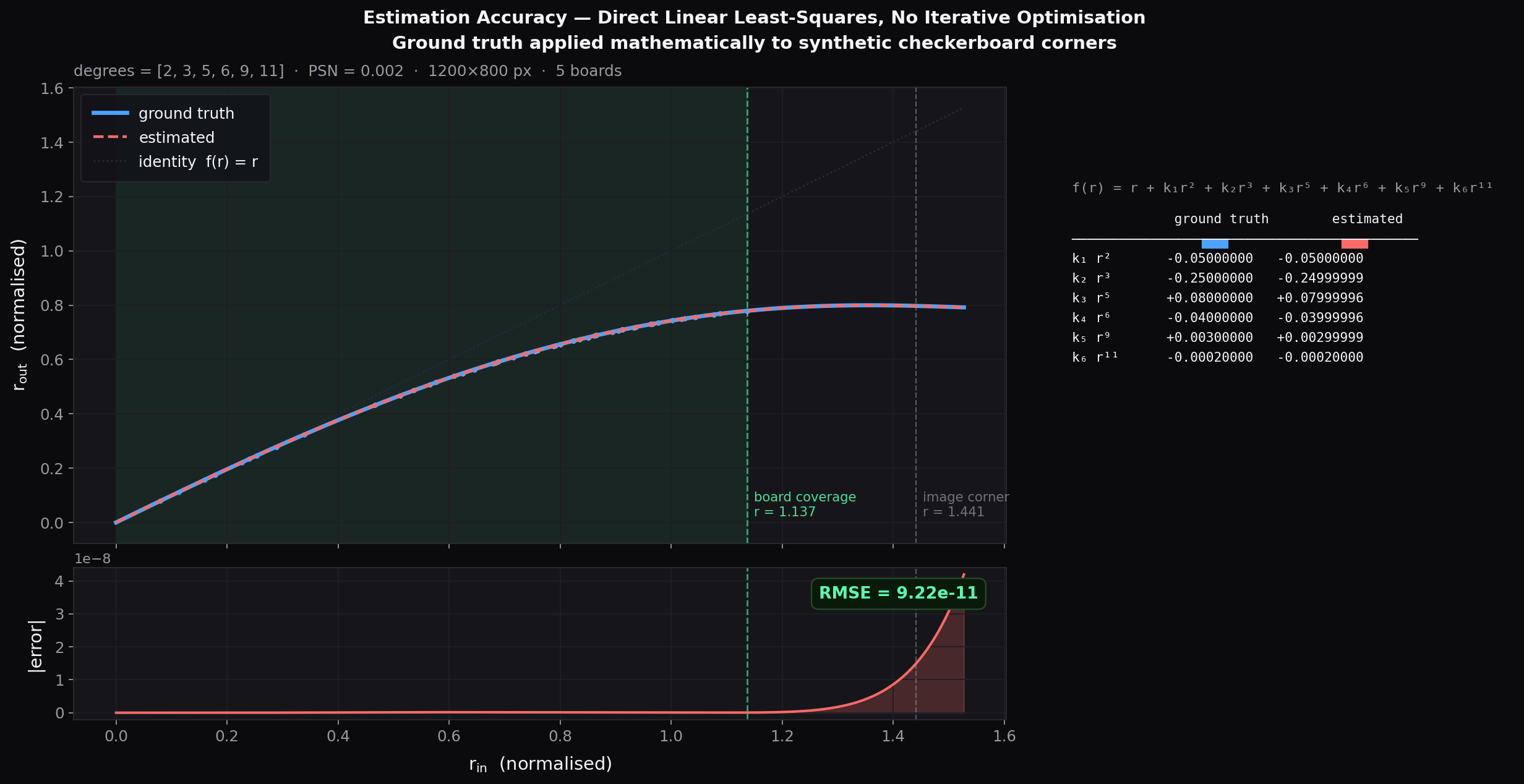
The distortion engine provides a controlled ground-truth test field:
a known analytical radial distortion model with known coefficients and known
radial behavior. The estimator is then evaluated against that ground truth.
It does not need to recover the same symbolic structure; it can use only the
required degrees and terms to reproduce the radial mapping across the covered field.
Ground truth: a strong barrel model, degrees [3, 5, 7, 9, 11]. The estimator
automatically selects a different, sparser set — degrees [2, 3, 4, 5] — and
reproduces the radial mapping to an RMSE of 4.0×10⁻⁵ out to the image
corner (five checkerboard boards spanning the full field). Calibration recovers
the distortion function over the observed range, not the original
coefficient set; coverage is reported alongside the result.
Automatic Degree Selection
Starting from r², the estimator adds polynomial terms one by one and
re-fits after each addition. It stops when RMSE drops below a user-defined
threshold — no manual model specification required.
Mixed Odd & Even Terms
Odd, even, sparse, and mixed-degree terms are all supported.
The model is not restricted to Brown–Conrady-style r³, r⁵, r⁷ terms — and
the same selection extends beyond polynomials to non-polynomial local bases.
See Function Freedom.
Deterministic Estimation
Each fit is a direct linear least-squares solve —
no iterative optimizer, no convergence loop, no initialization sensitivity.
Only the model structure grows; the fitting step stays deterministic.
Numerically Exact Undistortion
Both images below are undistorted with the estimated
coefficients — not the known ground truth — through a deterministic, precomputed
inverse. For monotonic mappings the recovered image matches the
original up to interpolation-grid and resampling effects. The
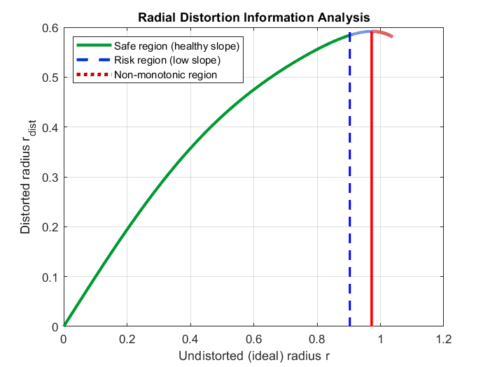
non-monotonic column uses a known distortion model that folds
at a fixed radius: past the fold, several scene points collapse onto the same
image radius, so that band is mathematically non-invertible — genuinely
irrecoverable for any method. The engine reports it (hard / soft loss) and
leaves it black in place rather than fabricating it; the frame is preserved,
not cropped or mirrored. Crucially, our estimator is monotonicity-constrained:
it never returns a non-monotonic model, so every recovered mapping is invertible
by construction and undistortion never silently folds.
Function Freedom: Beyond Fixed Distortion Families NEW
Real optics are not always a textbook barrel. Molded aspheric lenses carry
mid-spatial-frequency zonal ripple; foveated and panomorph designs
deliberately compress the periphery through a narrow transition. These are
smooth, strictly monotonic, physically valid mappings — but they lie outside
the span of the fixed families (Brown, rational, Kannala–Brandt) that standard
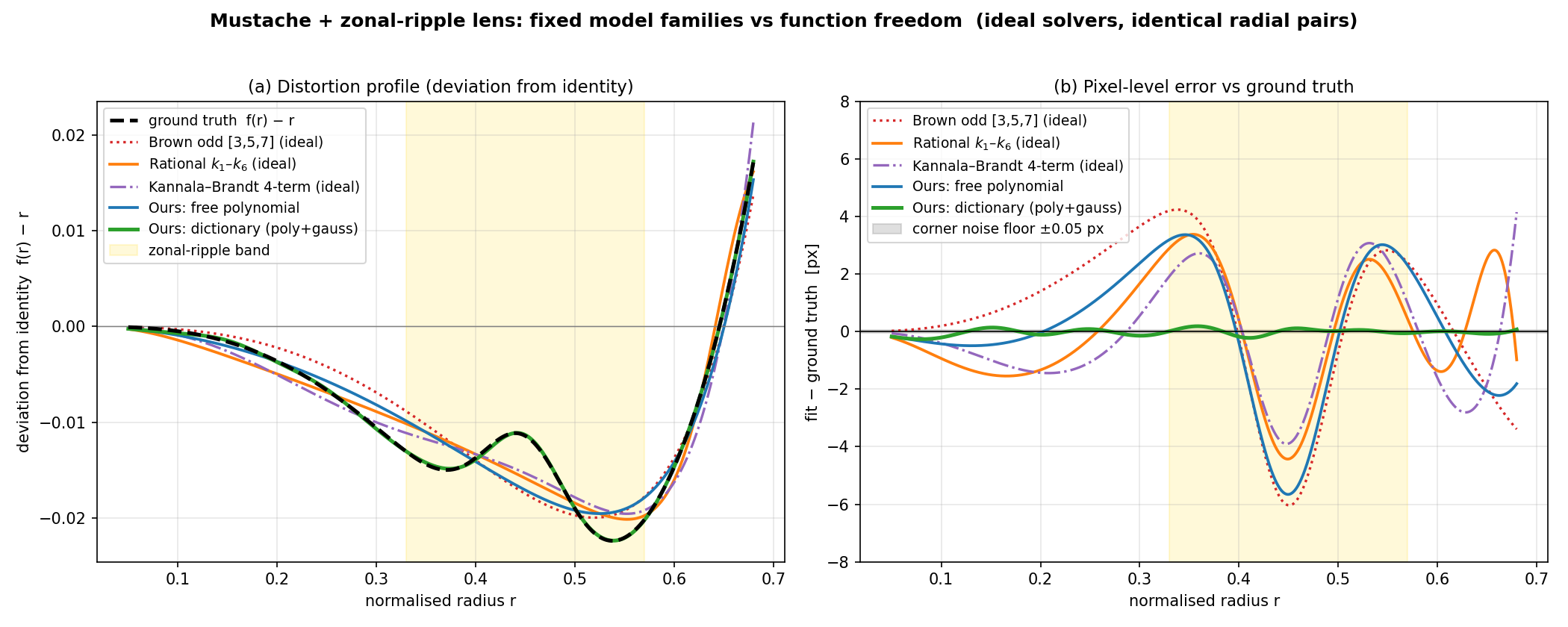
tools fit. On a zonal-ripple lens, even an ideal solver leaves those families
with multi-pixel error, while the same selection machinery over polynomial +
local bases reaches the corner-noise floor.
Zonal-ripple lens, ideal least-squares solvers on identical radial pairs.
Best fixed family (Kannala–Brandt): 4.16 px max error. Brown / rational:
4.4–6.0 px. A real OpenCV calibration: 47–70 px. Our dictionary
(polynomial + local bases): 0.26 px, at the noise floor —
a 16× gap. The estimated model is
f(r) = r + a·r² + b·r⁹ + Σ gᵢ·exp(−((r−cᵢ)/wᵢ)²),
and the selection places its first Gaussian term at c ≈ 0.45 —
exactly the radius of the zonal feature it was never told about.
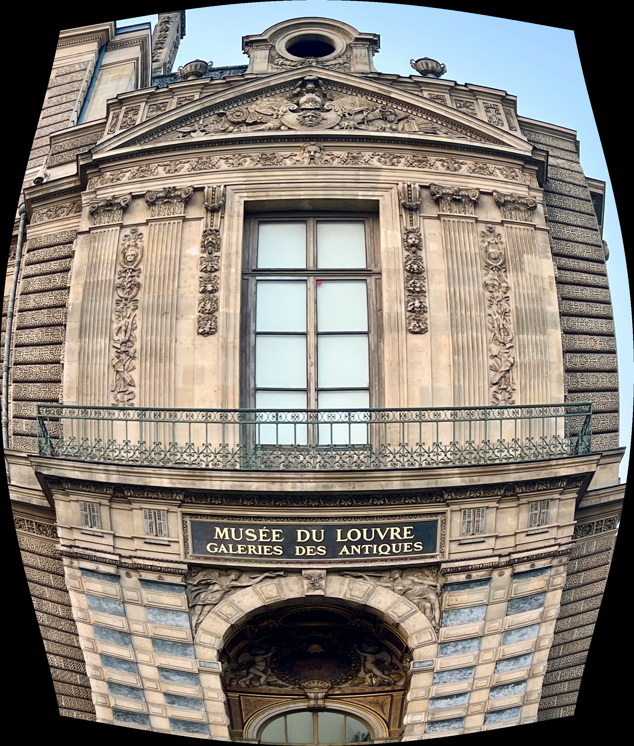
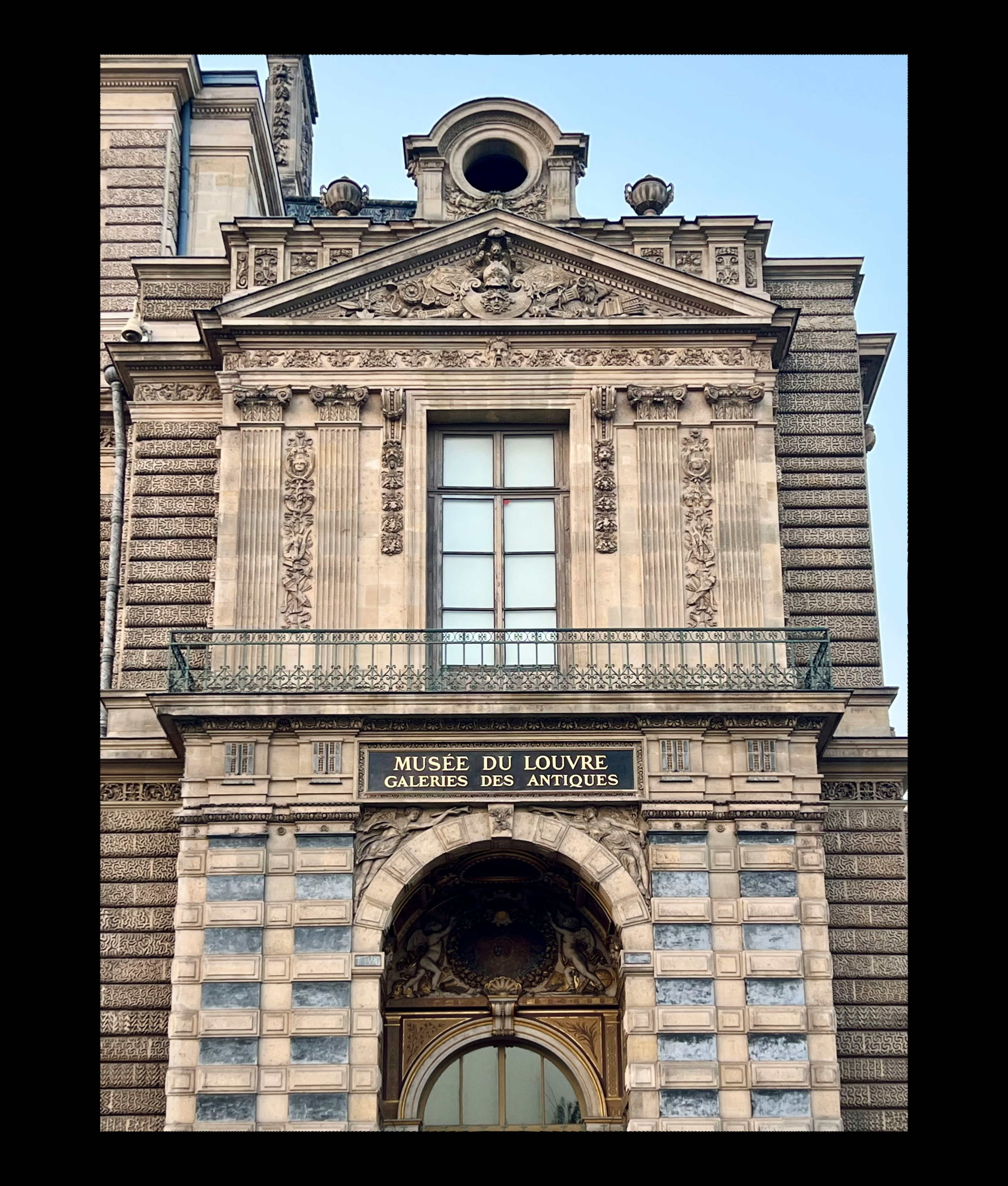
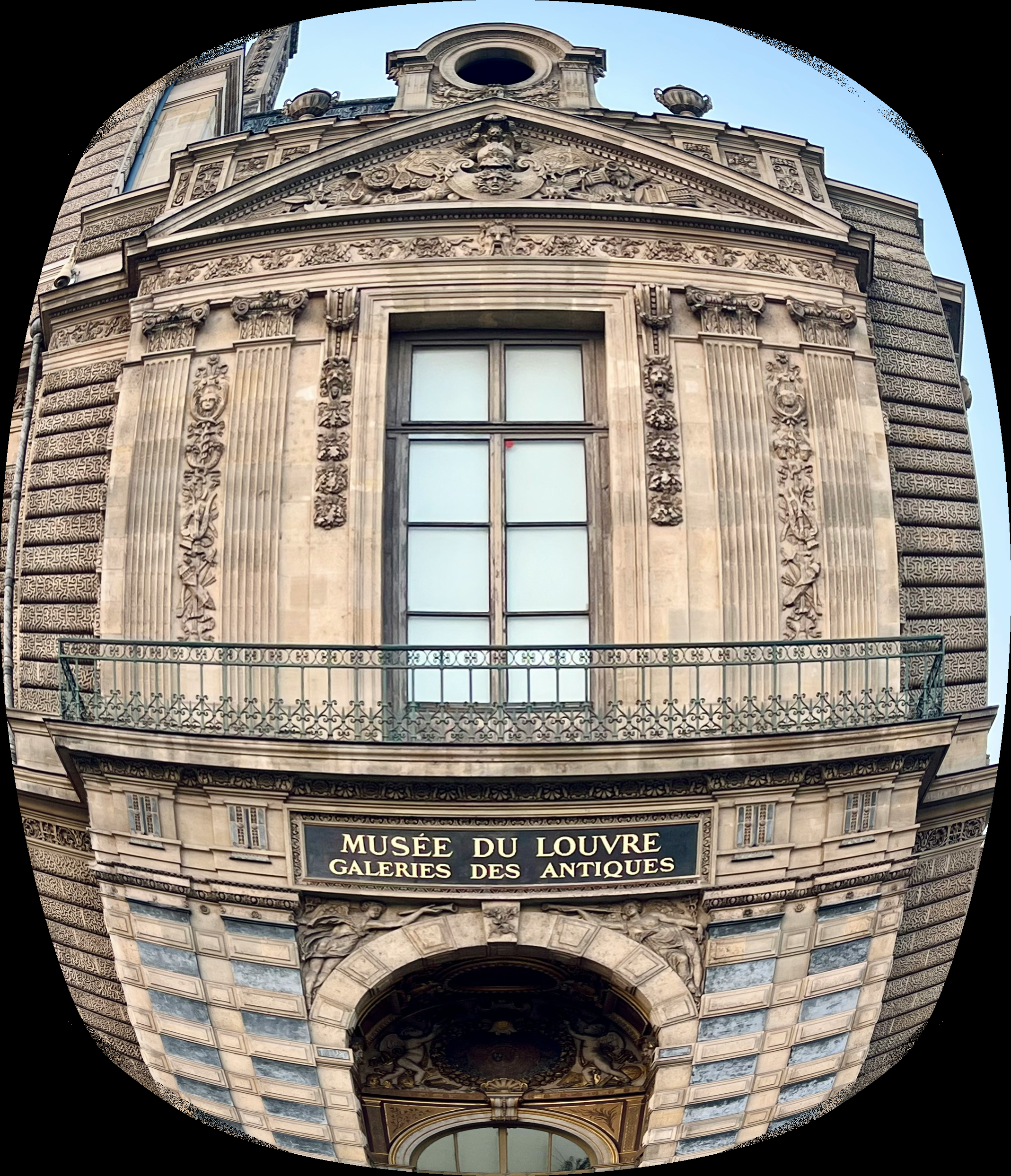
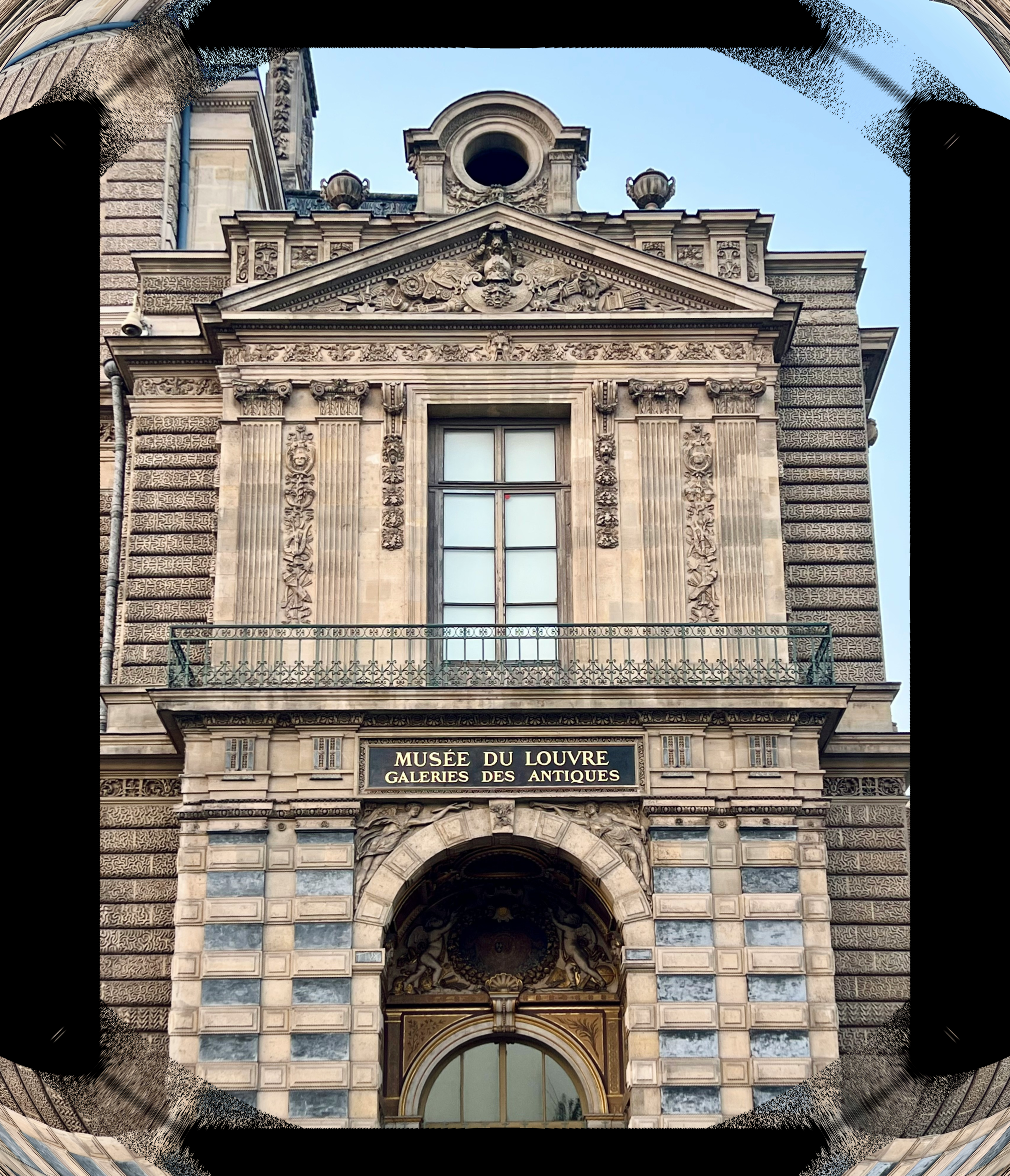
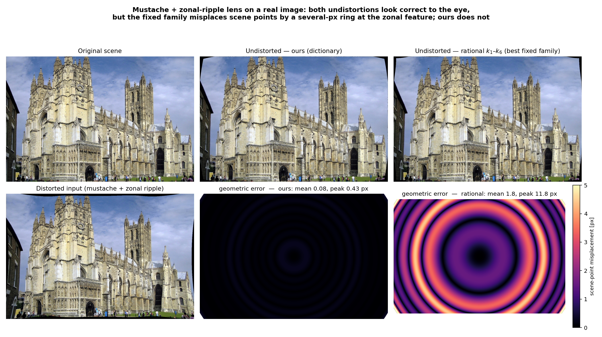
The Same Lens on a Real Image
Top: original scene, undistorted with our fit, undistorted with the best
fixed family — all three look correct to the eye. Bottom: the per-pixel
geometric error. The fixed family misplaces scene points by a bright ring
(mean 1.8 px, peak 11.8 px) at the zonal feature; our fit leaves
no structure (mean 0.08 px, peak 0.4 px). The error is invisible
in the picture yet would corrupt any downstream metrology at the affected
radii.
Polynomial + Local Bases
Gaussian zonal terms and sigmoid knees join the monomial basis. The
selection identifies the lens's own design parameters when they are present
(e.g. a knee at r = 0.55).
Constraint Always Holds
Every candidate basis term — polynomial or local — must keep the mapping
monotonic over the covered domain. Expressiveness never comes at the cost of
a physically invalid model.
Silent Failure, Made Visible
A fitted distortion model can fold — beyond the calibration coverage, or
when over-fitted, a polynomial often turns non-monotonic even if the lens is
not. A standard pipeline applies it to the whole frame and silently renders
mirrored content in the folded band, despite a sub-0.1 px reprojection
error. The engine checks monotonicity, undistorts the valid region, and flags
the folded band as hard loss instead of fabricating pixels.
Why The Recovery Is Different
Four design choices distinguish the engine from standard calibration and
undistortion workflows.
01 — Free Function Model
Arbitrary Degree, Terms & Bases
Polynomial degree and term count are fully user-defined — odd, even,
sparse, and mixed-degree terms. The same selection machinery extends to
non-polynomial local bases (Gaussian zonal terms, sigmoid knees),
representing real lens profiles that fixed global families cannot.
Standard tools commonly use fixed distortion families
and limited radial coefficient structures. See the
Function Freedom evidence above.
02 — Deterministic Calibration
Linear Least-Squares, Not Iterative Optimisation
Estimation is a direct linear solve for the distortion constants.
No Levenberg–Marquardt loop, no gradient descent, no local minima.
Standard tools typically minimize reprojection error
through iterative optimisation.
03 — Deterministic Inverse
Deterministic Inverse Mapping
The inverse is computed once and applied directly to every pixel —
no per-pixel iterative solver and no convergence loop.
Standard inverse workflows often rely on iterative
coordinate inversion.
04 — Physical Validity Control
Invertible by Construction
The estimator is monotonicity-constrained: it never returns a non-monotonic
(folding) model, so every recovered mapping is invertible and undistortion
never silently fabricates content. When a model is supplied externally, the
engine evaluates it for folding and quantifies irreversible (hard) vs.
recoverable (soft) loss before inversion.
Standard tools fit by reprojection error with no
monotonicity guard — an over-fitted or extrapolated model can fold, and they
do not report whether the mapping stays invertible over the field.
Estimate → Validate → Undistort
The workflow is intentionally explicit. The distortion function is not hidden
inside a black-box calibration result; it remains visible, inspectable, and
testable against known ground truth throughout the pipeline.
Checkerboard Images
Corner Detection (Harris + CNN)
Polynomial Recovery
Monotonicity Validation
Precomputed Inverse
Safe Undistortion
Automatic Model Selection
Starting from r², polynomial terms are added one by one and re-fitted
after each addition. The process stops when RMSE drops below a user-defined
threshold — the model grows only as complex as the data requires.
Multi-Board Pooling
Multiple checkerboards at different field positions can be combined
to improve radial coverage and estimation stability.
Classical & Learned Detection
Corners come from a built-in Harris detector or a trained
EfficientNet-V2-S + U-Net heatmap detector. The learned detector holds up
under strong barrel compression where gradient corners degrade, extending
usable radial coverage.
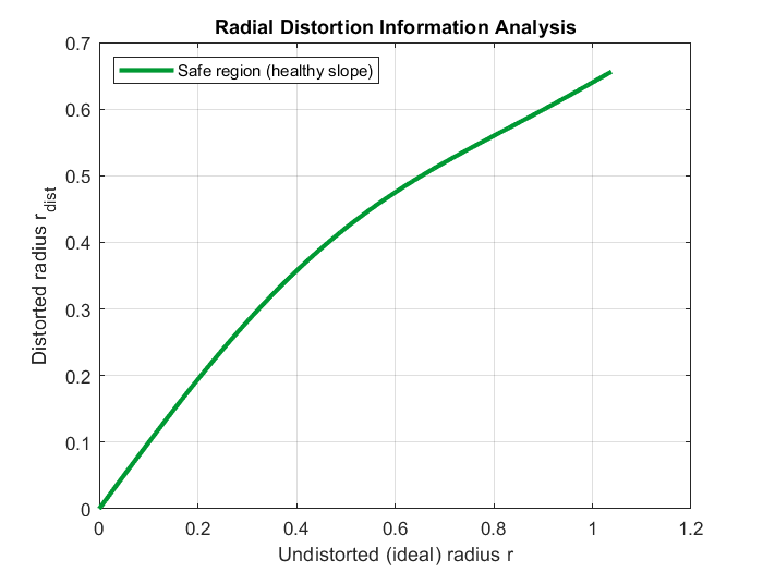
Monotonicity Validation
Before inversion, the estimated model is evaluated for folding and
information loss. Hard loss and soft loss ratios are reported explicitly.
Unified Distortion Engine
The same analytical forward-first framework is available as a MATLAB toolbox
and as a standalone Python package. The forward engine is used both as a
practical modeling tool and as a ground-truth generator for validation.
For research, ML pipelines, and large-scale synthetic dataset generation.
The core engine and Harris path have no required OpenCV dependency — built
on NumPy, SciPy, and Pillow. The optional learned corner detector adds
PyTorch and timm.
Commercial · Python
Roadmap & Future Work
Higher-Resolution Learned Detection
The EfficientNet-V2-S + U-Net corner detector ships today; training at
higher inference resolution and fine-tuning on real camera photographs will
push reliable coverage closer to the distortion fold.
Differential Calibration
Physically constrained differential calibration methods for
advanced optical systems.
Expanded Estimation Patterns
Line-based and synthetic image pair estimation, extending beyond
checkerboard patterns.
Licensing & Availability
Available as a MATLAB toolbox (.mltbx) and a Python package, under
commercial licenses for research and industrial use.
Research & Academic License
Suitable for universities, research groups, and individual researchers.
Commercial License
For industrial applications, product development, and internal tooling.
Evaluation Access
Limited evaluation versions available upon request.